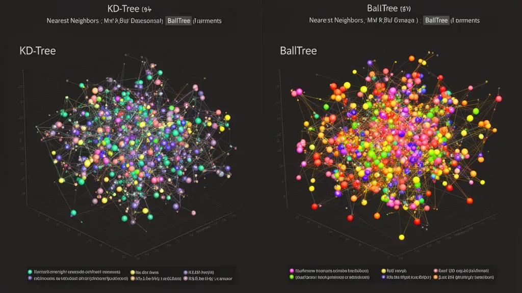
Spatial algorithms are at the heart of many computational problems, especially when dealing with multi-dimensional data. The scipy.spatial module in SciPy is packed with tools that allow you to efficiently manage and query spatial data. One of the fundamental structures you’ll encounter is the KD-tree, which is particularly useful for nearest neighbor searches.
from scipy.spatial import KDTree

data_points = [[1, 2], [3, 4], [5, 6], [7, 8]]
tree = KDTree(data_points)

# Query the nearest neighbor for the point (2, 3)
distance, index = tree.query([2, 3])
print("Nearest neighbor:", data_points[index], "at distance:", distance)
Another powerful structure is the BallTree, which is designed for high-dimensional data and can handle various distance metrics. That’s particularly useful when the standard Euclidean distance is not the most suitable choice for your data’s distribution.
from scipy.spatial import BallTree
import numpy as np

data_points = np.array([[1, 2], [3, 5], [4, 6], [8, 9]])
tree = BallTree(data_points)

# Query the nearest neighbor for the point (3, 4)
dist, ind = tree.query([3, 4])
print("Nearest neighbor:", data_points[ind], "at distance:", dist)
When working with spatial data, understanding the underlying algorithms can significantly enhance your ability to optimize performance. For example, the choice between KD-tree and BallTree can influence the efficiency of your queries based on the dimensionality of your data. As the number of dimensions increases, KD-trees can become inefficient, whereas BallTrees maintain their performance better in such scenarios.
from scipy.spatial import cKDTree

# Using cKDTree for faster performance with large datasets
data_points = np.random.rand(1000, 3)  # 1000 points in 3D
tree = cKDTree(data_points)

# Query for the nearest neighbors of a random point
query_point = np.random.rand(3)
distances, indices = tree.query(query_point, k=5)
print("Nearest neighbors:", data_points[indices], "at distances:", distances)
Another aspect worth noting is the integration of these spatial algorithms with other libraries, such as NumPy for efficient numerical operations. By using these tools, you can create robust applications for geographic information systems, computer graphics, and machine learning tasks that require spatial reasoning.
import matplotlib.pyplot as plt

# Visualizing points and their nearest neighbors
plt.scatter(data_points[:, 0], data_points[:, 1], color='blue')
for index in indices:
    plt.scatter(data_points[index, 0], data_points[index, 1], color='red')
plt.scatter(query_point[0], query_point[1], color='green', marker='x')  # Query point
plt.show()
Understanding these algorithms provides a solid foundation for building more complex systems. The efficiency of spatial queries can drastically improve with the right data structure, reducing computation time from linear to logarithmic in many cases. As you delve deeper into the capabilities of scipy.spatial, you’ll find that the performance gains are not merely theoretical but can be realized in practical applications.

PopSockets Adhesive Phone Grip, Holder, Phone Stand, Black - Black
$9.94 (as of July 16, 2026 15:11 GMT +00:00 - More infoProduct prices and availability are accurate as of the date/time indicated and are subject to change. Any price and availability information displayed on [relevant Amazon Site(s), as applicable] at the time of purchase will apply to the purchase of this product.)Implementing efficient data structures for spatial queries
To further enhance query performance, consider the use of spatial indexing techniques. Spatial indexing structures, such as R-trees, can significantly improve the efficiency of range queries and nearest neighbor searches. The R-tree organizes spatial data into a hierarchical structure, where each node contains bounding boxes that group nearby points together.
from scipy.spatial import cKDTree
from rtree import index

# Create an R-tree index
idx = index.Index()

# Insert points into the R-tree
for i, point in enumerate(data_points):
    idx.insert(i, (point[0], point[1], point[0], point[1]))

# Perform a range query
query_box = (2, 2, 5, 5)  # Define a bounding box
results = list(idx.intersection(query_box))
print("Points within the bounding box:", [data_points[i] for i in results])
Moreover, the choice of distance metrics can also play a pivotal role in optimizing spatial queries. For instance, when using the KD-tree or BallTree, you can specify different distance functions according to the nature of your data. This flexibility allows you to tailor the search process to yield better results based on your specific context.
from sklearn.neighbors import NearestNeighbors

# Using NearestNeighbors with a custom metric
nbrs = NearestNeighbors(n_neighbors=5, algorithm='ball_tree', metric='manhattan').fit(data_points)
distances, indices = nbrs.kneighbors([[2, 3]])
print("Nearest neighbors with Manhattan distance:", data_points[indices[0]], "at distances:", distances[0])
It is also essential to consider the dimensionality of your data when selecting an appropriate spatial data structure. As dimensionality increases, the curse of dimensionality can lead to inefficiencies. Therefore, it’s often beneficial to experiment with dimensionality reduction techniques, such as PCA, before applying spatial queries.
from sklearn.decomposition import PCA

# Reducing dimensions with PCA
pca = PCA(n_components=2)
reduced_data = pca.fit_transform(data_points)

# Building a KD-tree with reduced dimensionality
tree = KDTree(reduced_data)
distance, index = tree.query(pca.transform([[2, 3]]))
print("Nearest neighbor in reduced space:", reduced_data[index], "at distance:", distance)
As you implement these techniques, always keep in mind the trade-offs between accuracy and performance. While some algorithms may provide faster results, they might sacrifice precision. Conversely, more accurate methods could lead to longer processing times. Balancing these factors is important in developing efficient spatial query systems.
# Example of balancing speed and accuracy
from scipy.spatial import distance

# Function to compute the nearest neighbor with a trade-off
def query_with_tradeoff(tree, point, use_approximation=True):
    if use_approximation:
        return tree.query(point, k=1)  # Fast but may not be exact
    else:
        return tree.query(point, k=1, p=2)  # Exact computation

nearest = query_with_tradeoff(tree, [2, 3])
print("Nearest neighbor:", nearest)
To wrap it up, using advanced data structures and indexing techniques can drastically improve the performance of spatial queries. By understanding the strengths and weaknesses of each approach, you can design your systems to handle complex spatial operations efficiently, paving the way for innovative applications in various fields. As you continue to explore the capabilities of scipy.spatial and related libraries, you’ll discover numerous strategies for optimizing your spatial data processing tasks.
Optimizing performance with spatial indexing techniques
To further enhance query performance, consider the use of spatial indexing techniques. Spatial indexing structures, such as R-trees, can significantly improve the efficiency of range queries and nearest neighbor searches. The R-tree organizes spatial data into a hierarchical structure, where each node contains bounding boxes that group nearby points together.
from scipy.spatial import cKDTree
from rtree import index

# Create an R-tree index
idx = index.Index()

# Insert points into the R-tree
for i, point in enumerate(data_points):
    idx.insert(i, (point[0], point[1], point[0], point[1]))

# Perform a range query
query_box = (2, 2, 5, 5)  # Define a bounding box
results = list(idx.intersection(query_box))
print("Points within the bounding box:", [data_points[i] for i in results])
Moreover, the choice of distance metrics can also play a pivotal role in optimizing spatial queries. For instance, when using the KD-tree or BallTree, you can specify different distance functions according to the nature of your data. This flexibility allows you to tailor the search process to yield better results based on your specific context.
from sklearn.neighbors import NearestNeighbors

# Using NearestNeighbors with a custom metric
nbrs = NearestNeighbors(n_neighbors=5, algorithm='ball_tree', metric='manhattan').fit(data_points)
distances, indices = nbrs.kneighbors([[2, 3]])
print("Nearest neighbors with Manhattan distance:", data_points[indices[0]], "at distances:", distances[0])
It’s also essential to consider the dimensionality of your data when selecting an appropriate spatial data structure. As dimensionality increases, the curse of dimensionality can lead to inefficiencies. Therefore, it is often beneficial to experiment with dimensionality reduction techniques, such as PCA, before applying spatial queries.
from sklearn.decomposition import PCA

# Reducing dimensions with PCA
pca = PCA(n_components=2)
reduced_data = pca.fit_transform(data_points)

# Building a KD-tree with reduced dimensionality
tree = KDTree(reduced_data)
distance, index = tree.query(pca.transform([[2, 3]]))
print("Nearest neighbor in reduced space:", reduced_data[index], "at distance:", distance)
As you implement these techniques, always keep in mind the trade-offs between accuracy and performance. While some algorithms may provide faster results, they might sacrifice precision. Conversely, more accurate methods could lead to longer processing times. Balancing these factors is important in developing efficient spatial query systems.
# Example of balancing speed and accuracy
from scipy.spatial import distance

# Function to compute the nearest neighbor with a trade-off
def query_with_tradeoff(tree, point, use_approximation=True):
    if use_approximation:
        return tree.query(point, k=1)  # Fast but may not be exact
    else:
        return tree.query(point, k=1, p=2)  # Exact computation

nearest = query_with_tradeoff(tree, [2, 3])
print("Nearest neighbor:", nearest)
Using advanced data structures and indexing techniques can drastically improve the performance of spatial queries. By understanding the strengths and weaknesses of each approach, you can design your systems to handle complex spatial operations efficiently, paving the way for innovative applications in various fields. As you continue to explore the capabilities of scipy.spatial and related libraries, you’ll discover a high number of strategies for optimizing your spatial data processing tasks.